Chapters


Finding Measures of Central Tendency for Grouped Data
In previous sections introducing the concept of mean, median and mode, we discussed how descriptive statistics are generally divided between measures of central tendency and of variability. Here, we will expand upon what you learned about measures of central tendency by showing you how to calculate the mean, median and mode for grouped data.
Basic Measures of Central Tendency
Measures of central tendency are used to capture and describe the centre of a variable. They are employed when wanting to understand and illustrate the most “typical” value or values of a data set. In the table below, you’ll find a brief overview of these measures.
| Definition | Formula | Calculation | |
| Mean | The average \[ \bar{x} = \] \[ \frac{\Sigma x_{i}}{n} \] | (on the left) | 1. Add all the observations 2. Divide that summed value by the sample size, |
| Median | The midpoint of the data, where half the observations fall above and below | No standard formula | 1. Order the observations from least to greatest 2. Take the middle value 3. If the number of observations is even, take the average of the two middle values |
| Mode | The most occurring value of a variable | No standard formula | 1. Calculate the frequency of each value 2. The value with the highest frequency is the most occurring value, or the mode |
Grouped Data
So far, we’ve worked with data sets that list individual observations. This simply means that for each value, you can see each individual observation. For example, take the table below.
| Observation | Frequency |
| 60 | 1 |
| 61 | 3 |
| 62 | 2 |
| 63 | 5 |
| 64 | 7 |
| 65 | 2 |
| 66 | 1 |
Written out, this data would look like the following,
60, 61, 61, 61, 62, 62, 63, 63, 63, 63, 63, 64, 64, 64, 64, 64, 64, 64, 65, 65, 66
Here, finding the mean, median and mode is easy.
| Measure | Calculation |
| Mean | \[ = \frac{\Sigma}{n} = \dfrac{1326}{21} = 63.1 \] |
| Median | The midpoint of the data is 63 |
| Mode | The most occurring value in the data set is 64 |
However, data doesn’t always come packaged with the individual observations listed. In addition, sometimes you’re not necessarily interested in understanding individual data but rather groups within the data.
Grouped data is simply when observations are placed into groups, normally into intervals of some sort. Examples of grouped data include age groups, height groups, time groups and more. While categorical data can also be grouped, for example the frequency of each colour group in a paint store, grouped measures of central tendency make more intuitive sense when using only quantitative variables.
In the table below, you’ll find an example of grouped data for age groups.
| Age Groups | Frequency |
| 0 - 10 | 40 |
| 10 - 20 | 53 |
| 20 - 30 | 58 |
| 30 - 40 | 64 |
| 40 - 50 | 72 |
| 50 - 60 | 49 |
| 60 - 70 | 36 |
| 70 - 80 | 25 |
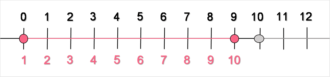
Keep in mind that in each group, only the first value, or the lower limit, of the interval is included up until the value before the upper limit, or the last value, of the group. Meaning, while 0 is included in the interval 0 through 10, 10 is not included. Instead, 9 is included, meaning there are 10 values in each group because we start counting at 0. Take a look at the image below for clarification.
Grouped Mean
Finding the grouped mean is easy. Simply, follow the formula below.
\[
x_{group} = \frac{\Sigma(f_{i}*x_{m})}{n}
\]
The table below contains the explanation of the notation.
| Element | Description |
 | Group mean |
 | The frequency of the  observation observation |
 | The midpoint of the x |
 | The sample size |
Using the example from above, we get the group mean performing the following steps.
| Age Groups | Frequency
| | * |
| 0 - 10 | 40 | \[ \dfrac{9+0}{2} = 4.5 \] | \[ 40 * 4.5 = 180 \] |
| 10 - 20 | 53 | 14.5 | 768.5 |
| 20 - 30 | 58 | 24.5 | 1421 |
| 30 - 40 | 64 | 34.5 | 2208 |
| 40 - 50 | 72 | 44.5 | 3204 |
| 50 - 60 | 49 | 54.5 | 2670.5 |
| 60 - 70 | 36 | 64.5 | 2322 |
| 70 - 80 | 25 | 74.5 | 1862.5 |
| Total | 397 | 14636.5 |
Plugging this into the formula, we get,
\[
x_{group} = \frac{14636.5}{397} = 36.9
\]
We attain 36.9, meaning that the mean is somewhere between 30 and 40.
Grouped Median
Similarly, finding the median for grouped data requires a different process. To find the group mean, you must follow the formula below.
\[
x_{med} = L + \frac{\frac{n}{2} - B}{G} * w
\]
The table below contains the explanation of the notation.
| Element | Description |
 | Group median |
 | The lower limit of the median group |
| The sample size |
 | The cumulative frequency of all groups below the median group |
 | The frequency of the group with the median |
 | The width of the groups |
Using the same example, we can see that the median of all the groups is roughly the middle point of the total frequency.
\[
\dfrac{397}{2} = 198.5
\]
The 199th point occurs somewhere in the group 30 - 40 (in reality 30 to 39). We can do this estimation because the data are in order.
The cumulative frequency can be found in the table below.
| Age Groups | Frequency
| |
| 0 - 10 | 40 | |
| 10 - 20 | 53 | \[ 40+53 = 93 \] |
| 20 - 30 | 58 | \[ 40+53+58 = 151 \] |
| 30 - 40 | 64 | 215 |
| 40 - 50 | 72 | 287 |
| 50 - 60 | 49 | 336 |
| 60 - 70 | 36 | 372 |
| 70 - 80 | 25 | 397 |
From the previous calculations, we get the following values.
| Element | Value |
| 30 |
| 397 |
| 151 |
| 64 |
| 10 |
Plugging these values into the formula, we get
\[
x_{med} = 30 + \frac{\frac{397}{2} - 151}{64} * 10 = 37.4
\]
Our estimate of the median is about 37.
Grouped Mode
The formula for the mode of grouped data is as follows.
\[
x_{mode} = L + \frac{ f_{m} - f_{m-1} }{ (f_{m} - f_{m-1}) + (f_{m} - f_{m+1}) } * w
\]
The table below contains the explanation of the notation.
| Element | Description |
 | Group mode |
| The lower limit of the group with the mode (the group with the highest frequency) |
 | Frequency of the group with the mode |
 | Frequency of the group before the one with the mode |
 | Frequency of the group after the one with the mode |
| The width of the groups |
Using the same example, we get the following.
| Element | Value |
| 40 |
| 72 |
| 64 |
| 49 |
| 10 |
Plugging this into the formula, we get
\[
x_{mode} = 40 + \frac{ 72 - 64 }{ (72 - 64) + (72 - 49) } * 10 = 42.6
\]
Which gives us a mode of about 43.
Practice Problem 1
Find the group mean of the following data.
| Scores | Frequency |
| 1-20 | 5 |
| 21 - 40 | 20 |
| 41 - 60 | 47 |
| 61 - 80 | 15 |
| 81 - 100 | 3 |
Practice Problem 2
Find the group mode of the following data.
| Students | Frequency |
| 1-3 | 135 |
| 4-6 | 457 |
| 7-9 | 549 |
| 10-12 | 392 |
Solution Problem 1
Follow the steps below to find the solution.
| Scores | Frequency | | * |
| 1-20 | 5 | \[ \dfrac{1+20}{2} = 10.5 \] | \[ 5 * 10.5 = 52.5 \] |
| 21 - 40 | 20 | 30.5 | 610 |
| 41 - 60 | 47 | 50.5 | 2373.5 |
| 61 - 80 | 15 | 70.5 | 1057.5 |
| 81 - 100 | 3 | 90.5 | 271.5 |
| 90 | 4365 |
\[
x_{group} = \frac{4365}{90} = 48.5
\]
The group mean is between 41 and 60.
Solution Problem 2
The estimation of the mode can be found by following the steps below.
| Element | Value |
| 7 |
| 549 |
| 457 |
| 392 |
| 3 |
\[
x_{mode} = 7 + \frac{ 549 - 457 }{ (549 - 457) + (549 - 392) } * 3 = 8.1
\]
Meaning the estimation of the mode is 8.1.
Did you like this article? Rate it!


Can you help me answer my activities